
gwpv
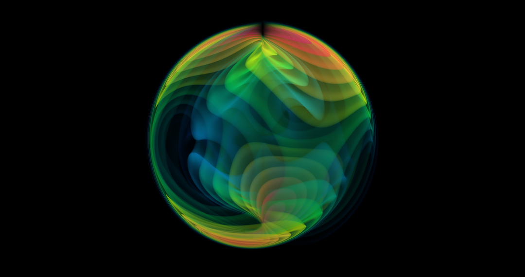
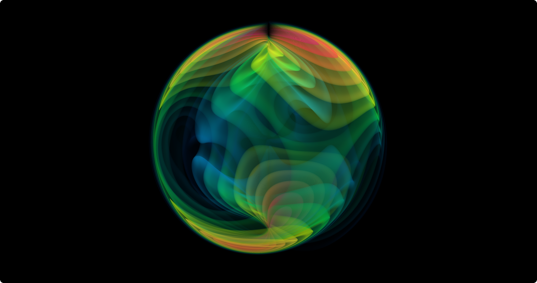
A visualization code for gravitational wave data I created in 2020 with Python and ParaView, published under the MIT license.
This Python package uses the ParaView scientific visualization toolkit to produce 3D renderings of gravitational wave data from a numerical simulation or a waveform model.
From README.md in the nilsvu/gwpv GitHub repository:
gwpv
This Python package uses the ParaView scientific visualization toolkit to produce 3D renderings of gravitational-wave data from a numerical simulation or a waveform model.
Try it now:
docker run -v $PWD:/out nilsleiffischer/gwpv:latest \
scene Examples/Rainbow/Still.yaml -o /out
Table of contents
- Installation
- Usage
- Explore waveform data in the ParaView GUI application
- Gallery
- Licensing and credits
Installation
Option 1: Pre-built Docker container
- Install Docker.
docker run nilsleiffischer/gwpv:latest
Docker will pull the latest pre-built image and run it. The container runs the
gwrender.py
entrypoint automatically (see Usage). To output rendered
frames and load data from your system you can mount directories using Docker’s
-v
option. Try rendering one of the example scenes:
docker run -v $PWD:/out nilsleiffischer/gwpv:latest \
scene Examples/Rainbow/Still.yaml -o /out
Here we mount the current working directory $PWD
as the directory /out
in
the container and use it to output frames. You can mount additional directories
to make your scene configuration files and data available in the container (see
Usage).
Option 2: Native environment
It is strongly recommended to use Python 3 for this program. In particular, parallel rendering may not work with Python 2 and setting up the environment with Python 3’s
venv
is more robust than Python 2’svirtualenv
.
- Install ParaView. Prefer versions with Python 3. This program was tested thoroughly with ParaView version 5.8.
- Create a virtual environment
with ParaView’s Python. With Python 3 you could do this:
path/to/python3 -m venv path/to/new/env
Make sure to set up the environment with the same Python installation that ParaView uses. If you are unsure, try this:
# Start interactive ParaView Python shell path/to/pvpython # Output path to the Python executable >>> import sys >>> sys.executable
On macOS the
pvpython
executable is typically located in/Applications/ParaView-X.Y.Z.app/Contents/bin
. The Python executable determined by the script above may be namedvtkpython
, in which case you can look for thepython2
orpython3
executable in the same directory or abin
subdirectory. - Give ParaView access to the environment. If you have created the environment
with Python 3’s
venv
then copy thescripts/activate_this.py
script to the environment:cp scripts/activate_this.py path/to/new/env/bin
Note that environments created with the
virtualenv
package include this script automatically and you don’t need to copy it. The script is used to activate the environment from within Python scripts. It allows ParaView’s Python to pick up the packages installed in the environment (see this blog post for details).You may also want to add the ParaView executables such as
pvpython
to yourPATH
when the environment is activated for convenient access. To do so you can append the following line topath/to/env/bin/activate
as well:export PATH="path/to/paraview/bin/:$PATH"
On macOS you may also need to append this line to pick up the
paraview
GUI executable:export PATH="path/to/paraview/MacOS/:$PATH"
- Install the following packages in the environment, making sure to use
ParaView’s HDF5 when installing
h5py
:. env/bin/activate HDF5_DIR=path/to/paraview/hdf5/ pip install --no-binary=h5py h5py pip install [-e] path/to/this/repository
Note that the
HDF5_DIR
should haveinclude
andlib
directories with ParaView’s HDF5. On macOS it is typically/Applications/ParaView-X.Y.Z.app/Contents/
. Add the-e
flag when installing this repository’s Python package to install it in “editable” mode, i.e. symlink instead of copy it so changes to the repository are reflected in the installation. On Python 2,pip install llvmlite==0.31.0
manually because later versions drop support for Python 2.
Usage
Try rendering one of the example scenes like this:
gwrender.py scene Examples/Rainbow/Still.yaml -o ./
The rendered scene is a still frame defined by the configuration file
Examples/Rainbow/Still.yaml
. It is based on
Examples/Rainbow/Rainbow.yaml
which, by
itself, defines a short movie:
gwrender.py scene Examples/Rainbow/Rainbow.yaml \
--render-movie-to-file ./Rainbow
--num-jobs NUM_JOBS
Feel free to turn up NUM_JOBS
to render the frames in parallel.
Compose configuration files to define a scene
A scene is defined by a stack of one or more YAML configuration files. The
configuration files can be source-controlled and shared, so each visualization
is reproducible. See
Examples/Rainbow/Rainbow.yaml
for an example
of a scene configuration file.
Multiple configuration files can be stacked to compose a scene. Configurations
in later files override those in earlier files. You find a collection of useful
configuration files in the directory scene_overrides/
.
They are found automatically by gwrender.py
, so you can, for example, easily
adjust the background of the scene or the rendering resolution:
gwrender.py \
scene Examples/Rainbow/Still.yaml Background/Light Resolutions/High -o ./
Scene configuration files can specify that they always include others so you don’t have to build the composition stack on the command line:
Include:
- Background/Light
- Resolutions/High
You can also list scene compositions in a file such as
Examples/Rainbow/Scenes.yaml
:
Scenes:
- Name: RainbowLight
Composition:
- Rainbow
- Background/Light
You can sequentially render all scenes listed in such a file by calling the
scenes
entrypoint:
gwrender.py scenes Examples/Rainbow/Scenes.yaml -o ./ --num-jobs NUM_JOBS
To render a single scene from the file, use the scene
entrypoint and specify
the name of the scene:
gwrender.py scene Examples/Rainbow/Scenes.yaml:Rainbow -o ./ --num-jobs NUM_JOBS
Sometimes it can be useful to override particular configurations from the
command line, for example to reduce the frame rate for a test rendering. To do
so, you can pass key-value pairs of scene configuration options to gwrender.py
like this:
gwrender.py scene Examples/Rainbow/Rainbow.yaml -o ./ \
--override Animation.FrameRate=1
The key of each override
is parsed as the key-path into the scene
configuration to replace, and its value is parsed as YAML.
Datasources
To specify datasources for the rendered scenes, such as waveform data or horizon
shapes from a simulation, the configuration file
Examples/Rainbow/Rainbow.yaml
includes
Examples/Rainbow/Datasources.yaml
.
Specifying the datasources in a separate configuration file allows excluding it from source control, e.g. to set local file system paths on a particular rendering machine.
Datasources can refer to a local file system path or a remote URL. They will be downloaded and cached, if needed. For example, you can pick any simulation from the SXS waveform catalog and use the URL to one of its public waveform data files:
Datasources:
Waveform:
File: https://zenodo.org/record/3321679/files/Lev3/rhOverM_Asymptotic_GeometricUnits_CoM.h5
Subfile: Extrapolated_N2.dir
Cache: ./waveform_data_cache
Explore waveform data in the ParaView GUI application
- We need to make ParaView aware of our Python environment and the plugins in
this repository. This is easiest done from the command line. Before launching
the ParaView GUI, make sure the Python environment is activated as described
in Installation. Then launch ParaView like this:
PV_PLUGIN_PATH=path/to/paraview_plugins path/to/paraview
You will now find the plugins provided by this repository in the ParaView GUI when you select ‘Tools’ > ‘Manage Plugins’.
- Open a waveform data file in ParaView and select the Waveform Data Reader to load it. Waveform data files in SpEC’s output format are currently supported.
- Add the Waveform To Volume filter to the loaded data.
- Change the representation to Volume and adjust the following properties:
- Volume Rendering Mode (try GPU Based and enable Shade)
- Scalar Opacity Unit Distance (try a quarter of the domain size)
- Transfer function (select Edit color map)
Gallery
Here’s a few images and movies produces with this software package:
GW190412
- Source: nilsleiffischer/gw190412-movie
- More information and images available at: https://www.aei.mpg.de/214403/gw190412-binary-black-hole-merger and https://dcc.ligo.org/LIGO-G2000575/public
-
Video:
- Selected media coverage:
- https://www.nature.com/articles/d41586-020-01153-7
- https://www.sciencenews.org/article/gravitational-waves-unevenly-sized-black-holes-ligo-virgo
- https://www.aei.mpg.de/213678/a-signal-like-none-before
- https://www.ligo.org/detections/GW190412
- https://www.ligo.caltech.edu/news/ligo20200420
- https://www.spektrum.de/news/neuartiges-gravitationswellensignal/1725506
GW190814
- Source: nilsleiffischer/gw190814-movie
- More information and images available at: https://www.aei.mpg.de/263744/gw190814 and https://dcc.ligo.org/LIGO-G2000730/public
-
Video:
- Selected media coverage:
- https://www.aei.mpg.de/267070/a-black-hole-with-a-puzzling-companion
- https://www.ligo.org/detections/GW190814
- https://www.space.com/smallest-black-hole-biggest-neutron-stary-mystery-object.html
- https://www.dailymail.co.uk/sciencetech/article-8451939/Mysterious-cosmic-object-lighter-black-hole-heavier-neutron-star-discovered.html
GW190521
- Source: nilsleiffischer/gw190521-movie
- More information and images available at: https://www.aei.mpg.de/500856/gw190521 and https://dcc.ligo.org/LIGO-G2001282/public
-
Video:
- Selected media coverage:
- https://www.aei.mpg.de/296843/ligo-and-virgo-catch-their-biggest-fish-so-far
- https://www.ligo.caltech.edu/news/ligo20200902
- https://aasnova.org/2020/09/02/ligo-virgos-newest-merger/
Licensing and credits
This code is distributed under the MIT license. Please see the
LICENSE
for details. When you use code from this project or
publish media produced by this code, please include a reference back to the
nilsleiffischer/gwpv repository.
Copyright (c) 2020 Nils Leif Fischer